
One of the successful insights to training neural networks has been the rectified linear unit, or short the ReLU, as a fast alternative to the traditional activation functions such as the sigmoid or the tanh. One of the major advantages of the simle ReLu is that it does not saturate at the upper end, thus the network is able to distinguish a poor answer from a really poor answer and correct accordingly.
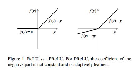
A modification to the ReLU, the Leaky ReLU, that would not saturate in the opposite direction has been tested but did not help. Interestingly in a recent paper by the Microsoft© deep learning team, He et al. revisited the subject and introduced a Parametric ReLU, the PReLU, achieving superhuman performance on the imagenet. The PReLU learns the parameter α (alpha) and adjusts it through basic gradient descent.
In this tutorial I will benchmark a few different implementations of the ReLU and PReLU together with Theano. The benchmark test will be on the MNIST database, mostly for convenience.
Why Theano
Coming from an R environment I tried to find a good deep learning alternative in R. Unfortunately the graphics card integration is often lacking and it seems that the other alternatives are much further along. I chose Theano as this is one of the most popular packages and it compiles everything at the back-end for speed. There are several packages that build upon Theano but I figured it was just as well to learn something from the core.
Possible ReLU and PReLU implementations
I’ve come across a few different ReLU implementations:
1 2 3 4 5 6 7 8 9 10 11 12 13 14 | def ReLU1(X): return T.maximum(X, 0.) def ReLU2(X): return T.switch(X < 0., 0., X) def ReLU3(X): return ((X + abs(X)) / 2.0) def ReLU4(X): return X * (X > 0) def ReLU5(X): return (T.sgn(X) + 1) * X * 0.5 |
The only one that is slightly less intuitive is the third one where the the absolute causes the value to cancel out while the positive values are divided by one half. For obvious reasons only the ReLU2 and ReLU3 are possible to adapt to a PReLU version:
1 2 3 4 5 6 7 | def PReLU2(X, alpha): return T.switch(X < 0, alpha * X, X) def PReLU3(X, alpha): pos = ((X + abs(X)) / 2.0) neg = alpha * ((X - abs(X)) / 2.0) return pos + neg |
Note that this also requires the alpha parameters for the PReLU set. These need to correspond to the number of activations in the corresponding layer and be included in the update function – here’s an abstract of the PReLU test function that takes care of this. Note the calculations of the input sizes and how they relate as this is crucial for setting the correct alpha shapes:
1 2 3 4 5 6 7 8 9 10 11 12 13 14 15 16 17 18 19 20 21 22 23 24 25 26 27 28 29 30 31 32 33 | # Input size from MNIST: 28 x 28 pixels # First filter gives (28 + 3 - 1, 28 + 3 -1) = (30, 30) # - note the full border alternative # The maxpool (2,2) gives (15, 15) # The output is thus (32, 15, 15) product = 7200 w1 = init_weights((32, 1, 3, 3)) # Second filter gives (15 - 3 + 1, 15 - 3 + 1) = (13, 13) # The maxpool (2,2) gives (7, 7) # - note that maxpool has ignore_border = False by default # The output is thus (64, 7, 7) product = 3136 w2 = init_weights((64, 32, 3, 3)) # Third filter gives (7 - 3 + 1, 7 - 3 + 1) = (5, 5) # The maxpool (2,2) gives (3, 3) # The output is thus (128, 3, 3) product = 1152 w3 = init_weights((128, 64, 3, 3)) # Note that the 3 is not the filter size above w4 = init_weights((128 * 3 * 3, 625)) # The fully connected layer sizes are rather straight forward w_o = init_weights((625, 10)) alpha1 = theano.shared(np.ones((30,), dtype=theano.config.floatX)*.5) alpha2 = theano.shared(np.ones((13,), dtype=theano.config.floatX)*.5) alpha3 = theano.shared(np.ones((5,), dtype=theano.config.floatX)*.3) alpha4 = theano.shared(np.ones((625,), dtype=theano.config.floatX)*.1) params = [w1, w2, w3, w4, w_o, # Note the addition of the alpha to the update alpha1, alpha2, alpha3, alpha4] updates = RMSprop(cost, params, lr=0.001) |
Setting up the MNIST
I rely on the excellent tutorial by Alec Radford for loading the MNIST database:
1 2 3 4 5 | from load import mnist trX, teX, trY, teY = mnist(onehot=True) trX = trX.reshape(-1, 1, 28, 28) teX = teX.reshape(-1, 1, 28, 28) |
As the MNIST is almost too easy we’ll limit the dataset to 1/6 of the original size:
1 2 3 4 | # Reduce the sample in order to make the problem a little harder select = np.random.choice(trX.shape[0], 10000, replace=False) trX = trX[select,:] trY = trY[select,:] |
The basic ReLU benchmark functions
The network is identical to that of Alec’s original net that attains about 99.5% accuracy on the full dataset after 30 epochs.
1 2 3 4 5 6 7 8 9 10 11 12 13 14 15 16 17 18 19 20 21 22 23 24 25 26 27 28 29 30 31 32 33 34 35 36 37 38 39 40 41 42 43 44 45 46 47 48 49 50 51 52 53 54 55 56 57 58 59 60 61 62 63 64 65 66 67 68 69 70 71 72 73 74 75 76 77 78 79 80 81 82 83 84 85 86 87 88 89 90 91 92 93 94 95 96 97 98 99 100 | def runModelTraining(epochs, train, predict, alpha1 = None, alpha2 = None, alpha3 = None, alpha4 = None): block_size = 128 i = 0 top_accuracy = 0 start_time = time.time() duration = [] accuracy = [] while i < epochs: i = i + 1 for start in range(0, trY.shape[0], block_size): end = start + block_size if (end > trY.shape[0]): end = trY.shape[0] train(trX[start:end], trY[start:end]) # Print basic output print "** Run no. {0} **".format(i) duration.append(getDuration(start_time)) accuracy.append(testAccuracy(test_x=teX, test_y=teY, predict_fn=predict)) print "With a {accuracy:.2f}% accuracy".format(accuracy= accuracy[len(accuracy) - 1]* 100) # For the alphas we want to make sure that they learn something if (not alpha1 == None): print "The alpha values are for " +\ " no. 1: {alpha1:.2f}, no. 2: {alpha2:.2f}".format(alpha1 = np.mean(alpha1.get_value()), alpha2 = np.mean(alpha2.get_value())) + \ " no. 3: {alpha3:.2f} , no. 4: {alpha4:.2f}".format(alpha3 = np.mean(alpha3.get_value()), alpha4 = np.mean(alpha4.get_value())) return duration, accuracy def ReLU_eval(activator, epochs = no_epochs): # Create tensor variables that will be used in the models X = T.ftensor4() Y = T.fmatrix() # Input size from MNIST: 28 x 28 pixels # First filter gives (28 + 3 - 1, 28 + 3 -1) = (30, 30) # - note the full border alternative # The maxpool (2,2) gives (15, 15) # The output is thus (32, 15, 15) product = 7200 w1 = init_weights((32, 1, 3, 3)) # Second filter gives (15 - 3 + 1, 15 - 3 + 1) = (13, 13) # The maxpool (2,2) gives (7, 7) # - note that maxpool has ignore_border = False by default # The output is thus (64, 7, 7) product = 3136 w2 = init_weights((64, 32, 3, 3)) # Third filter gives (7 - 3 + 1, 7 - 3 + 1) = (5, 5) # The maxpool (2,2) gives (3, 3) # The output is thus (128, 3, 3) product = 1152 w3 = init_weights((128, 64, 3, 3)) # Note that the 3 is not the filter size above w4 = init_weights((128 * 3 * 3, 625)) # The fully connected layer sizes are rather straight forward w_o = init_weights((625, 10)) def basic_model(X, w1, w2, w3, w4, w_o, p_drop_conv, p_drop_hidden, activator): l1a = activator(conv2d(X, w1, border_mode='full')) l1 = max_pool_2d(l1a, (2, 2)) l1 = dropout(l1, p_drop_conv) l2a = activator(conv2d(l1, w2)) l2 = max_pool_2d(l2a, (2, 2)) l2 = dropout(l2, p_drop_conv) l3a = activator(conv2d(l2, w3)) l3b = max_pool_2d(l3a, (2, 2)) l3 = T.flatten(l3b, outdim=2) l3 = dropout(l3, p_drop_conv) l4 = activator(T.dot(l3, w4)) l4 = dropout(l4, p_drop_hidden) pyx = softmax(T.dot(l4, w_o)) return pyx noise_py_x = basic_model(X = X, w1 = w1, w2 = w2, w3 = w3, w4 = w4, w_o = w_o, p_drop_conv = 0.2, p_drop_hidden = 0.5, activator = activator) py_x = basic_model(X = X, w1 = w1, w2 = w2, w3 = w3, w4 = w4, w_o = w_o, p_drop_conv = 0., p_drop_hidden = 0., activator = activator) y_x = T.argmax(py_x, axis=1) cost = T.mean(T.nnet.categorical_crossentropy(noise_py_x, Y)) params = [w1, w2, w3, w4, w_o] updates = RMSprop(cost, params, lr=0.001) train = theano.function(inputs=[X, Y], outputs=cost, updates=updates, allow_input_downcast=True) predict = theano.function(inputs=[X], outputs=y_x, allow_input_downcast=True) duration, accuracy = runModelTraining(epochs, train, predict) return duration, accuracy |
The PReLU training is identical with a few small exceptions:
1 2 3 4 5 6 7 8 9 10 11 12 13 14 15 16 17 18 19 20 21 22 23 24 25 26 27 28 29 30 31 32 33 34 35 36 37 38 39 40 41 42 43 44 45 46 47 48 49 50 51 52 53 54 55 56 57 58 59 60 61 62 63 64 65 66 67 68 69 70 71 72 73 74 75 76 77 78 79 80 81 82 | def PReLU_eval(activator, epochs = no_epochs): # Create tensor variables that will be used in the models X = T.ftensor4() Y = T.fmatrix() # Input size from MNIST: 28 x 28 pixels # First filter gives (28 + 3 - 1, 28 + 3 -1) = (30, 30) # - note the full border alternative # The maxpool (2,2) gives (15, 15) # The output is thus (32, 15, 15) product = 7200 w1 = init_weights((32, 1, 3, 3)) # Second filter gives (15 - 3 + 1, 15 - 3 + 1) = (13, 13) # The maxpool (2,2) gives (7, 7) # - note that maxpool has ignore_border = False by default # The output is thus (64, 7, 7) product = 3136 w2 = init_weights((64, 32, 3, 3)) # Third filter gives (7 - 3 + 1, 7 - 3 + 1) = (5, 5) # The maxpool (2,2) gives (3, 3) # The output is thus (128, 3, 3) product = 1152 w3 = init_weights((128, 64, 3, 3)) # Note that the 3 is not the filter size above w4 = init_weights((128 * 3 * 3, 625)) # The fully connected layer sizes are rather straight forward w_o = init_weights((625, 10)) alpha1 = theano.shared(np.ones((30,), dtype=theano.config.floatX)*.5) # @UndefinedVariable alpha2 = theano.shared(np.ones((13,), dtype=theano.config.floatX)*.5) # @UndefinedVariable alpha3 = theano.shared(np.ones((5,), dtype=theano.config.floatX)*.3) # @UndefinedVariable alpha4 = theano.shared(np.ones((625,), dtype=theano.config.floatX)*.1) # @UndefinedVariable def basic_model(X, w1, w2, w3, w4, w_o, alpha1, alpha2, alpha3, alpha4, p_drop_conv, p_drop_hidden, activator): l1a = activator(conv2d(X, w1, border_mode='full'), alpha1) l1 = max_pool_2d(l1a, (2, 2)) l1 = dropout(l1, p_drop_conv) l2a = activator(conv2d(l1, w2), alpha2) l2 = max_pool_2d(l2a, (2, 2)) l2 = dropout(l2, p_drop_conv) l3a = activator(conv2d(l2, w3), alpha3) l3b = max_pool_2d(l3a, (2, 2)) l3 = T.flatten(l3b, outdim=2) l3 = dropout(l3, p_drop_conv) l4 = activator(T.dot(l3, w4), alpha4) l4 = dropout(l4, p_drop_hidden) pyx = softmax(T.dot(l4, w_o)) return pyx noise_py_x = basic_model(X = X, w1 = w1, w2 = w2, w3 = w3, w4 = w4, w_o = w_o, alpha1 = alpha1, alpha2 = alpha2, alpha3 = alpha3, alpha4 = alpha4, p_drop_conv = 0.2, p_drop_hidden = 0.5, activator = activator) py_x = basic_model(X = X, w1 = w1, w2 = w2, w3 = w3, w4 = w4, w_o = w_o, alpha1 = alpha1, alpha2 = alpha2, alpha3 = alpha3, alpha4 = alpha4, p_drop_conv = 0., p_drop_hidden = 0., activator = activator) y_x = T.argmax(py_x, axis=1) cost = T.mean(T.nnet.categorical_crossentropy(noise_py_x, Y)) params = [w1, w2, w3, w4, w_o, # Note the addition of the alpha to the update alpha1, alpha2, alpha3, alpha4] updates = RMSprop(cost, params, lr=0.001) train = theano.function(inputs=[X, Y], outputs=cost, updates=updates, allow_input_downcast=True) predict = theano.function(inputs=[X], outputs=y_x, allow_input_downcast=True) duration, accuracy = runModelTraining(epochs, train, predict, alpha1 = alpha1, alpha2 = alpha2, alpha3 = alpha3, alpha4 = alpha4) return duration, accuracy |
Results and conclusions
My three main conclusions are:
- The maximum and the absolute calculations seem to have performed equally fast.
- The added time using PReLU is minimal.
- Similarly the added precision is minimal, although PReLU seems to slightly faster find the sweet-spot.
The latter point is hard to really on due to the limited complexity of the MNIST database, I would expect that PReLU comes in handy when dealing with more complex tasks.
Using some R-code I created a few plots illustrating the above conclusions (after some googling and getting an error when installing the python ggplot I gave up):
1 2 3 4 5 6 7 8 9 10 11 12 13 14 15 16 17 18 19 20 21 22 | fn <- "~/test/PReLU_benchmark.csv" df % group_by(grp, dur, epochs) %>% summarise(max = max(value), min = min(value), ratio = max/min) -> sum_df library(ggplot2) dur_df % group_by(Type, epochs) %>% summarise(avg = mean(value)) png(filename = "PReLU_acc_benchmark.png", width = 600*2, height = 400*2, res = 126) ggplot(acc_df, aes(x = epochs, y = avg, col = Type)) + geom_line(lwd = 2) + scale_y_continuous(lim = c(.3, 1), expand = c(0,0)) + scale_x_continuous(lim = c(4, 30), expand = c(0,0), breaks = seq(5, 30, by=5)) + scale_color_brewer(type = "qual", palette = 4) + guides(linetype = guide_legend(title = "Calc.")) + xlab("Epochs") + ylab("Accuracy") + theme_bw() + theme(text = element_text(size = 18)) dev.off() |


The α values
Interestingly the α (alpha) values behaved in a similar fashion to that in the original article, alphas in the lower layers were higher compared to lower layers. Here’s a shortened sample from the PReLU3 print:
Testing PReLU3
** Run no. 1 **
It took 7.7seconds
With a 12.29% accuracy
The alpha values are for  no. 1: 0.50, no. 2: 0.50 no. 3: 0.30 , no. 4: 0.10
** Run no. 2 **
It took 17.8seconds
With a 25.59% accuracy
The alpha values are for  no. 1: 0.50, no. 2: 0.50 no. 3: 0.30 , no. 4: 0.10
** Run no. 3 **
It took 27.9seconds
With a 21.56% accuracy
The alpha values are for  no. 1: 0.50, no. 2: 0.50 no. 3: 0.30 , no. 4: 0.10
** Run no. 4 **
It took 38.0seconds
With a 9.81% accuracy
The alpha values are for  no. 1: 0.50, no. 2: 0.50 no. 3: 0.30 , no. 4: 0.10
** Run no. 5 **
It took 48.1seconds
With a 43.79% accuracy
The alpha values are for  no. 1: 0.50, no. 2: 0.50 no. 3: 0.33 , no. 4: 0.10
** Run no. 6 **
It took 58.2seconds
With a 81.48% accuracy
The alpha values are for  no. 1: 0.51, no. 2: 0.52 no. 3: 0.36 , no. 4: 0.11
** Run no. 7 **
It took 1.0min, 8.3seconds
With a 93.87% accuracy
The alpha values are for  no. 1: 0.52, no. 2: 0.53 no. 3: 0.37 , no. 4: 0.11
** Run no. 8 **
It took 1.0min, 18.4seconds
With a 94.96% accuracy
The alpha values are for  no. 1: 0.53, no. 2: 0.53 no. 3: 0.37 , no. 4: 0.11
** Run no. 9 **
It took 1.0min, 28.5seconds
With a 96.49% accuracy
The alpha values are for  no. 1: 0.53, no. 2: 0.54 no. 3: 0.37 , no. 4: 0.11
** Run no. 10 **
It took 1.0min, 38.6seconds
With a 96.63% accuracy
The alpha values are for  no. 1: 0.54, no. 2: 0.54 no. 3: 0.37 , no. 4: 0.10
....
** Run no. 15 **
It took 2.0min, 29.1seconds
With a 97.67% accuracy
The alpha values are for  no. 1: 0.55, no. 2: 0.54 no. 3: 0.36 , no. 4: 0.10
....
** Run no. 20 **
It took 3.0min, 19.6seconds
With a 98.16% accuracy
The alpha values are for  no. 1: 0.56, no. 2: 0.54 no. 3: 0.35 , no. 4: 0.09
....
** Run no. 25 **
It took 4.0min, 10.1seconds
With a 98.04% accuracy
The alpha values are for  no. 1: 0.57, no. 2: 0.54 no. 3: 0.34 , no. 4: 0.09
** Run no. 26 **
It took 4.0min, 20.2seconds
With a 97.95% accuracy
The alpha values are for  no. 1: 0.57, no. 2: 0.54 no. 3: 0.34 , no. 4: 0.09
** Run no. 27 **
It took 4.0min, 30.3seconds
With a 98.37% accuracy
The alpha values are for  no. 1: 0.57, no. 2: 0.54 no. 3: 0.35 , no. 4: 0.09
** Run no. 28 **
It took 4.0min, 40.4seconds
With a 98.45% accuracy
The alpha values are for  no. 1: 0.57, no. 2: 0.54 no. 3: 0.35 , no. 4: 0.09
** Run no. 29 **
It took 4.0min, 50.5seconds
With a 98.43% accuracy
The alpha values are for  no. 1: 0.58, no. 2: 0.54 no. 3: 0.35 , no. 4: 0.09
** Run no. 30 **
It took 5.0min, 0.6seconds
With a 98.32% accuracy
The alpha values are for  no. 1: 0.58, no. 2: 0.54 no. 3: 0.34 , no. 4: 0.09
Deriving the ReLU/PReLU
Part of the speed impacting the implementation is the derivative. From what I understand this is something that Theano does in the background using the grad-function:
1 2 3 4 5 6 | import theano from theano import tensor as T from theano import pp x = T.dscalar('x') y = x ** 2 pp(T.grad(y, x)) |
Give the somewhat harder to read 2 * x:
((fill((x ** TensorConstant{2}), TensorConstant{1.0}) * TensorConstant{2}) *
  (x ** (TensorConstant{2} - TensorConstant{1})))
Using the same approach for the maximum function gives:
1 2 | y = T.maximum(x, 0) pp(T.grad(y, x)) |
It is readable but hardly intuitive that the meaning is x > 0 ? 1 : 0:
(eq(maximum(x, TensorConstant{0}), x) *
 fill(maximum(x, TensorConstant{0}), TensorConstant{1.0}))
The absolute calculation ((x + abs(x)) / 2.0) gives the rather mindnumming that I think reduces to (1 / 2 + 1 / 2 * x / |x|):
((fill(((x + |x|) / TensorConstant{2.0}), TensorConstant{1.0}) /
    TensorConstant{2.0}) +
   (((fill(((x + |x|) / TensorConstant{2.0}), TensorConstant{1.0}) /
        TensorConstant{2.0}) * x) /
      |x|))
And if your want to get a real headache, here’s the PReLU winner and it’s two derivatives:
1 2 3 4 5 6 7 | alpha = T.dscalar('alpha') pos = ((x + abs(x)) / 2.0) neg = alpha * ((x - abs(x)) / 2.0) y = neg + pos print(pp(T.grad(y, x))) print("\n") print(pp(T.grad(y, alpha))) |
I haven’t even tried to deduce the elements… not sure I can even find x > 0 ? 1 : α in this mess…
(((((fill(((\alpha * ((x - |x|) / TensorConstant{2.0})) +
             ((x + |x|) / TensorConstant{2.0})),
          TensorConstant{1.0}) *
       \alpha) / TensorConstant{2.0}) +
     (((-((fill(((\alpha * ((x - |x|) / TensorConstant{2.0})) +
                   ((x + |x|) / TensorConstant{2.0})),
                TensorConstant{1.0}) *
             \alpha) / TensorConstant{2.0})) *
         x) / |x|)) +
    (fill(((\alpha * ((x - |x|) / TensorConstant{2.0})) +
             ((x + |x|) / TensorConstant{2.0})),
          TensorConstant{1.0}) / TensorConstant{2.0})) +
   (((fill(((\alpha * ((x - |x|) / TensorConstant{2.0})) +
              ((x + |x|) / TensorConstant{2.0})),
           TensorConstant{1.0}) / TensorConstant{2.0}) *
       x) / |x|))


(fill(((\alpha * ((x - |x|) / TensorConstant{2.0})) +
         ((x + |x|) / TensorConstant{2.0})),
      TensorConstant{1.0}) *
   ((x - |x|) / TensorConstant{2.0}))
Environment
The benchmark was performed on a cuDNN-enabled K40c GPU together with Theano 0.7 and Ubuntu 14.04.
![]()